Project: Tracking ETF Holdings with Async Data Loading and TimeScaleDB

Exploring Ark ETFs: Harnessing a Time Series database for Dynamic Analysis and Visualization of large-scale time series data

Dec 08, 2023

I came across an interesting phenomena with actively managed ETFs like those marketed by ‘Ark Invest‘, where stocks tend to gain a sudden increase in volume and price after being added to a large ETF. For example back in Jan. 2021, ARKG added NNOX to its portfolio and in one day of trading between Jan. 25 and Jan. 26 it jumped ~40%.

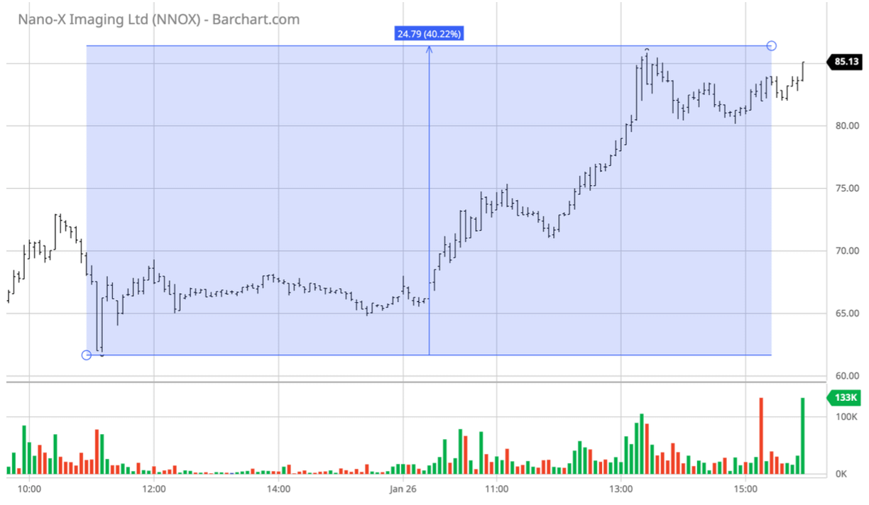
I wanted to be able to dynamically track the thousands of stocks and millions of daily price point data generated by Ark ETF holdings data so that I could take advantage of these price swings as soon as they happened. In order to do this, I built a relational database using TimeScaleDB developed off of PostgreSQL to store my price data on nearly 31k securities, which I populated using an async data loading script. I also wrote queries to explore some of SQL and PostgreSQL’s built-in analysis tools on my data.

Finally, I implemented a Streamlit dashboard where users can easily query this data and see the price analysis + visualizations for each stock in the database.

You can find my data and code at this Github repo: Ark-ETF-Tracker-Repo

Set-up

Why TimeScaleDB?

Using TimescaleDB for storing both time-series and non-time-series data gave me several distinct advantages over a regular PostgreSQL database. TimescaleDB is purpose-built for handling time-series data efficiently within the PostgreSQL ecosystem.

Its key benefits include optimized storage, indexing, and querying capabilities tailored specifically for time-series data. This resulted in drastic improvements in query response times, offering a more streamlined and performant experience. By leveraging hypertables and time-based partitioning, TimescaleDB excels in managing large volumes of time-stamped data, allowing faster and more performant queries, especially when dealing with historical stock price information.

The integration with PostgreSQL also enabled the storage of non-time-series data within the same database, such as symbols and exchange names, providing a unified platform for my stock-related data while maintaining the scalability and performance needed for time-series analytics.

Docker Image

I initially developed my TimescaleDB database using the official Docker image which streamlined setup. It eliminated the need to manually install and configure dependencies since Docker encapsulated the entire database setup, making it portable and consistent across various environments. When deploying on cloud platforms like AWS or GCP, Docker simplifies the process by allowing integration with cloud container services like ECS, EKS, or GKE.

Database Design

In order to prevent storing redundant and replicative data, I designed the following schema for my relational database tables. It includes a ‘stock‘ table to store basic information about publicly listed stocks/ETFs, an ‘etf_holding‘ table to store the specific holdings and weight allocations of each holding in my stored ETFs, and a ‘stock_price‘ table with 5-minute interval price bar data for each stock.

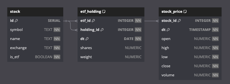
The ‘stock’ table serves as a fundamental repository for my stock information, storing unique identifiers (id) for each stock along with essential details like stock symbols, names, and the exchanges they are listed on. The ‘is_etf’ column acts as a marker denoting whether a particular stock is an ETF or not. The primary key (id) serves as the basis for foreign key references in other tables like ‘etf_holding’ and ‘stock_price’.

CREATE TABLE stock (
    id SERIAL PRIMARY KEY,
    symbol TEXT NOT NULL,
    name TEXT NOT NULL,
    exchange TEXT NOT NULL,
    is_etf BOOLEAN NOT NULL
);

Next, ‘etf_holding’ establishes relationships between ETFs and their constituent holdings (holding_id), linking them via foreign keys (etf_id). The table also records the date (dt) of these holdings along with the quantities of shares and their respective weights. The foreign key constraints ensure that the etf_id and holding_id values correspond to existing entries in the ‘stock’ table (id), maintaining data integrity and preventing invalid references.

CREATE TABLE etf_holding (
    etf_id INTEGER NOT NULL,
    holding_id INTEGER NOT NULL,
    dt DATE NOT NULL,
    shares NUMERIC,
    weight NUMERIC,
    PRIMARY KEY (etf_id, holding_id, dt),
    CONSTRAINT fk_etf FOREIGN KEY (etf_id) REFERENCES stock (id),
    CONSTRAINT fk_holding FOREIGN KEY (holding_id) REFERENCES stock (id)
);

Finally, ‘stock_price’ maintains price data for stocks in the form of 5-minute price bars. The ‘stock_id’ field links each price entry to a specific stock using a foreign key referencing the id column in the ‘stock’ table. This relationship enables the association of price data with corresponding stocks, ensuring accuracy and consistency in the representation of historical prices.

CREATE TABLE stock_price (
    stock_id INTEGER NOT NULL,
    dt TIMESTAMP WITHOUT TIME ZONE NOT NULL,
    open NUMERIC NOT NULL,
    high NUMERIC NOT NULL,
    low NUMERIC NOT NULL,
    close NUMERIC NOT NULL,
    volume NUMERIC NOT NULL,
    PRIMARY KEY (stock_id, dt),
    CONSTRAINT fk_stock FOREIGN KEY (stock_id) REFERENCES stock (id)
);

CREATE INDEX ON stock_price (stock_id, dt DESC);

SELECT create_hypertable('stock_price', 'dt');

I used those foreign key constraints to help maintain database integrity by enforcing referential integrity rules. This ensured that data inserted into the ‘etf_holding’ and ‘stock_price’ tables must correspond to existing entries in the ‘stock’ table.

When populating and querying the tables, this prevented orphaned records, maintained consistency, and avoided referencing non-existent data which safeguarded the coherence and reliability of the database.

Async Data Loading

When populating my ‘stock’ and ‘etf_holding’ tables, I created a database connection and cursor using Psycopg2 to interface with my database and execute SQL commands to load the required data.

# POPULATE STOCK TABLE

# connect to db
connection = psycopg2.connect(host=config.DB_HOST, database=config.DB_NAME, user=config.DB_USER, password=config.DB_PASS)

cursor = connection.cursor(cursor_factory=psycopg2.extras.DictCursor)

api = tradeapi.REST(config.API_KEY, config.API_SECRET, base_url=config.API_URL)

assets = api.list_assets()

for asset in assets:
    print(f"Inserting {asset.name} {asset.symbol}")
    cursor.execute("""
        INSERT INTO stock (name, symbol, exchange, is_etf)
        VALUES(%s, %s, %s, false)
    """, (asset.name, asset.symbol, asset.exchange))

connection.commit()

The following script connected my cursor to my database and searched through my .csv data file to find all the individual stock holdings and stock weights into the etf_holding table.

# POPULATE ETF_HOLDING TABLE

# connect to db
connection = psycopg2.connect(host=config.DB_HOST, database=config.DB_NAME, user=config.DB_USER, password=config.DB_PASS)

cursor = connection.cursor(cursor_factory=psycopg2.extras.DictCursor)

cursor.execute("select * from stock where is_etf=TRUE")

etfs = cursor.fetchall()

current_date = '2023-11-25'

for etf in etfs:
    print(etf['symbol'])

    with open(f"data/2023-11-25/{etf['symbol']}.csv") as f:
        reader = csv.reader(f)
        next(reader)
        for row in reader:
            ticker = row[3]

            if ticker:
                shares = row[5].replace(',', '')
                weight = row[7].replace('%', '')

                cursor.execute("""SELECT * FROM stock WHERE symbol = %s""", (ticker,))
                stock = cursor.fetchone()
                if stock:
                    cursor.execute(""" INSERT INTO etf_holding (etf_id, holding_id, dt, shares, weight) VALUES (%s, %s, %s, %s, %s)""",
                    (etf['id'], stock['id'], current_date, shares, weight))
connection.commit()

However, my price data was much larger as it included the open, high, low, close, for thousands of securities in 5 minute intervals. I wanted to explore more efficient and faster methods for populating my stock_prices table.

To do this I developed a script that utilised asynchronous programming with asyncio, aiohttp for HTTP requests, and asyncpg for asynchronous database interactions.

Here is a brief breakdown of how the coroutines and functions work asynchronously, with the full code at the bottom of this section.

Asynchronous Database Writing

async def write_to_db(connection, params):
    await connection.copy_records_to_table('stock_price', records=params)

The ‘write_to_db’ function handles the asynchronous writing of records to the database. It uses the asyncpg library's ‘copy_records_to_table’ method to efficiently insert records into the 'stock_price' table.

Fetching Price Data

async def get_price(pool, stock_id, url):
    try:
        async with pool.acquire() as connection:
            async with aiohttp.ClientSession() as session:
                async with session.get(url=url) as response:
                    resp = await response.read()
                    response = json.loads(resp)
                    params = [(stock_id, datetime.datetime.fromtimestamp(bar['t'] / 1000.0), round(bar['o'], 2), round(bar['h'], 2), round(bar['l'], 2), round(bar['c'], 2), bar['v']) for bar in response['results']]
                    await write_to_db(connection, params)
    except Exception as e:
        print("Unable to get url {} due to {}.".format(url, e.__class__))

The get_price function is responsible for fetching stock price data asynchronously. It utilizes an HTTP GET request using aiohttp to retrieve data from the specified URL. Upon receiving the response, it processes the JSON data, constructs parameter values, and writes them to the database asynchronously using the write_to_db function.

Concurrent Price Retrieval

async def get_prices(pool, symbol_urls):
    try:
        ret = await asyncio.gather(*[get_price(pool, stock_id, symbol_urls[stock_id]) for stock_id in symbol_urls])
        print("Finalized all. Returned list of {} outputs.".format(len(ret)))
    except Exception as e:
        print(e)

The get_prices function manages concurrent execution of get_price for multiple symbols using asyncio.gather. It triggers asynchronous requests for fetching stock prices, collecting all outputs, and printing the final count of outputs.

Stock Data Retrieval and Processing

async def get_stocks():
    pool = await asyncpg.create_pool(user=config.DB_USER, password=config.DB_PASS, database=config.DB_NAME, host=config.DB_HOST, command_timeout=60)
    
    async with pool.acquire() as connection:
        stocks = await connection.fetch("SELECT * FROM stock WHERE id IN (SELECT holding_id FROM etf_holding)")

        symbol_urls = {}
        for stock in stocks:
            symbol_urls[stock['id']] = f"https://api.polygon.io/v2/aggs/ticker/{stock['symbol']}/range/5/minute/2023-01-01/2023-11-01?adjusted=true&sort=asc&limit=120&apiKey='API_KEY'"

    await get_prices(pool, symbol_urls)

The get_stocks function creates a database connection pool using asyncpg.create_pool and fetches stock data from the database. It constructs symbol URLs for each stock and initiates the retrieval of their respective prices using get_prices.

Execution and Timing

start = time.time()
asyncio.run(get_stocks())
end = time.time()
print("Took {} seconds.".format(end - start))

The code initializes the execution by running the get_stocks coroutine within an asyncio.run call. It measures the elapsed time for the entire asynchronous process.

Full Script

import config
import json
import requests
import datetime, time
import aiohttp, asyncpg, asyncio


async def write_to_db(connection, params):
    await connection.copy_records_to_table('stock_price', records=params)


async def get_price(pool, stock_id, url):
    try: 
        async with pool.acquire() as connection:
            async with aiohttp.ClientSession() as session:
                async with session.get(url=url) as response:
                    resp = await response.read()
                    response = json.loads(resp)
                    params = [(stock_id, datetime.datetime.fromtimestamp(bar['t'] / 1000.0), round(bar['o'], 2), round(bar['h'], 2), round(bar['l'], 2), round(bar['c'], 2), bar['v']) for bar in response['results']]
                    await write_to_db(connection, params)

    except Exception as e:
        print("Unable to get url {} due to {}.".format(url, e.__class__))


async def get_prices(pool, symbol_urls):
    try:
        # schedule aiohttp requests to run concurrently for all symbols
        ret = await asyncio.gather(*[get_price(pool, stock_id, symbol_urls[stock_id]) for stock_id in symbol_urls])
        print("Finalized all. Returned  list of {} outputs.".format(len(ret)))
    except Exception as e:
        print(e)


async def get_stocks():
    # create database connection pool
    pool = await asyncpg.create_pool(user=config.DB_USER, password=config.DB_PASS, database=config.DB_NAME, host=config.DB_HOST, command_timeout=60)
    
    # get a connection
    async with pool.acquire() as connection:
        stocks = await connection.fetch("SELECT * FROM stock WHERE id IN (SELECT holding_id FROM etf_holding)")

        symbol_urls = {}
        for stock in stocks:
            # 5 min price bars from Jan 1 2023 - Nov 1 2023
            symbol_urls[stock['id']] = f"https://api.polygon.io/v2/aggs/ticker/{stock['symbol']}/range/5/minute/2023-01-01/2023-11-01?adjusted=true&sort=asc&limit=120&apiKey=IyLEoMj6Ms39XVhSW4SeLF6WZl9BO8XZ"

    await get_prices(pool, symbol_urls)


start = time.time()

asyncio.run(get_stocks())

end = time.time()

print("Took {} seconds.".format(end - start))

Data Analysis and Trend Detection

Now that my database was created and all my tables were loaded, I could begin to explore the holdings of each of the different Ark ETFs. I also wanted to explore the different built-in analysis functions from both standard PostgreSQL and TimeScaleDB.

These trends are detected for each stock held by each of the ETFs that I am tracking in order to add some technical indicators to my analysis.

Aggregating Daily Highs, Lows, and Closing Prices

-- high and low value of a stock for that day
SELECT max(high) FROM stock_price WHERE stock_id = 15117;
SELECT min(low) FROM stock_price WHERE stock_id = 15117;

-- closing price
SELECT last(close, dt) FROM stock_price WHERE stock_id = 15117;

To retrieve daily high and low values for a specific stock (stock_id = 15117), the queries calculate the maximum high (max(high)) and minimum low (min(low)) prices within the given date range. Additionally, the last recorded closing price (last(close, dt)) for that stock is obtained from the database.

Identifying Low Volume Stocks Held by Ark ETFs

SELECT stock_id, symbol, sum(volume) AS total_volume FROM stock_price JOIN stock ON stock.id = stock_price.stock_id GROUP BY stock_id, symbol ORDER BY total_volume ASC LIMIT 10;

This SQL query fetches stocks and their associated symbols, computing the total volume of their transactions. The result is sorted in ascending order by total volume, limited to the top 10 low-volume stocks held by Ark ETFs.

Creating Histogram with Specific Price Intervals

SELECT histogram(close, 19, 20, 4) FROM stock_price WHERE stock_id = 27104;

This query generates a histogram by categorizing the closing prices between $19 and $20 into four equal intervals, providing a distribution of stock prices within that range.

Aggregating Price Data into Custom Time Intervals

SELECT time_bucket(INTERVAL '1 hour', dt) AS bucket, first(open, dt), max(high), min(low), last(close, dt) 
FROM stock_price 
WHERE stock_id = 27104 
GROUP BY bucket 
ORDER BY bucket DESC;

SELECT time_bucket(INTERVAL '20 minute', dt) AS bucket, first(open, dt), max(high), min(low), last(close, dt) 
FROM stock_price 
WHERE stock_id = 27104 
GROUP BY bucket 
ORDER BY bucket DESC;

The provided queries utilize the time_bucket function to aggregate stock price data (open, high, low, close) based on specific time intervals (1 hour and 20 minutes) for a particular stock (stock_id = 27104). These aggregate results are grouped by the specified time intervals.

Filling Time Gaps and Missing Prices

SELECT time_bucket_gapfill('5 min', dt, now() - INTERVAL '5 day', now()) AS bar, 
avg(close) as close FROM stock_price WHERE stock_id = 7502 and dt > now () - INTERVAL '5 day' 
GROUP BY bar, stock_id ORDER BY bar;

This query uses time_bucket_gapfill to fill forward time gaps and missing prices for a specific stock (stock_id = 7502) within the last 5 days. It groups data into 5-minute intervals, calculating the average closing price per interval.

Creating Materialized Views for Aggregated Bars

CREATE MATERIALIZED VIEW hourly_bars WITH (timescaledb.continuous) AS 
SELECT stock_id, time_bucket(INTERVAL '1 hour', dt) AS day, 
first(open, dt) as open, MAX(high) as high, MIN(low) as low, 
last(close, dt) as close, SUM(volume) as volume 
FROM stock_price GROUP BY stock_id, day;

CREATE MATERIALIZED VIEW daily_bars WITH (timescaledb.continuous) AS 
SELECT stock_id, time_bucket(INTERVAL '1 day', dt) AS day, 
first(open, dt) as open, MAX(high) as high, MIN(low) as low,
last(close, dt) as close, SUM(volume) as volume 
FROM stock_price GROUP BY stock_id, day;

Two materialized views (hourly_bars and daily_bars) are created to pre-compute hourly and daily price bars by aggregating data from 5-minute bars. These views store aggregated information such as opening, high, low, closing prices, and volume for different time intervals.

Daily Moving Average

SELECT avg(close) FROM (
    SELECT * FROM daily_bars WHERE stock_id = 27104 ORDER BY day DESC LIMIT 20
) a;

This query computes the average closing price for a specific stock (stock_id = 27104) over the last 20 days. It selects the latest 20 entries from the daily_bars materialized view ordered by date in descending order and calculates their average closing price.

Identifying Daily Top Gainers

WITH prev_day_closing AS (
    SELECT stock_id, day, close, 
    LEAD(close) OVER (PARTITION BY stock_id ORDER BY day DESC) AS rev_day_closing_price 
    FROM daily_bars
), daily_factor AS ( 
    SELECT stock_id, day, close / prev_day_closing_price AS daily_factor 
    FROM prev_day_closing
) SELECT day, LAST(stock_id, daily_factor) AS stock_id, MAX(daily_factor) AS max_daily_factor 
FROM daily_factor 
JOIN stock ON stock.id = daily_factor.stock_id 
GROUP BY day 
ORDER BY day DESC, max_daily_factor DESC;

This query identifies the top gainers for each day by computing the daily factor, which is the ratio of the current day's closing price to the previous day's closing price. It then selects the day and the stock with the maximum daily factor, sorting the results in descending order of the daily factor.

Bullish Engulfing Pattern

SELECT * FROM (
    SELECT day, open, close, stock_id, LAG(close, 1) OVER ( PARTITION BY stock_id ORDER BY day ) previous_close, 
    LAG(open, 1) OVER ( PARTITION BY stock_id ORDER BY day ) previous_open 
    FROM daily_bars
) a 
WHERE previous_close < previous_open AND close > previous_open AND open < previous_close AND day = '2023-11-25';

This query aims to identify a bullish engulfing pattern within the daily_bars data for a specific day ('2023-11-25'). It examines the relationship between the previous day's close, open, and the current day's close and open to determine whether the day exhibits a bullish engulfing pattern.

The bullish engulfing pattern is a candlestick pattern that occurs when a larger bullish candlestick completely engulfs the previous smaller bearish candlestick.

This query checks if the previous day's closing price was lower than its opening price (previous_close < previous_open).
It confirms if the current day's closing price is higher than its opening price (close > previous_open).
It verifies if the current day's opening price is lower than the previous day's closing price (open < previous_close).

Higher Closing Price on Higher Volume

SELECT * FROM (
    SELECT day, close, volume, stock_id, LAG(close, 1) OVER ( PARTITION BY stock_id ORDER BY day ) previous_close, 
    LAG(volume, 1) OVER ( PARTITION BY stock_id ORDER BY day ) previous_volume, 
    LAG(close, 2) OVER ( PARTITION BY stock_id ORDER BY day ) previous_previous_close, 
    LAG(volume, 2) OVER ( PARTITION BY stock_id ORDER BY day ) previous_previous_volume 
    FROM daily_bars
) a 
WHERE close > previous_close AND previous_close > previous_previous_close AND volume > previous_volume 
AND previous_volume > previous_previous_volume AND day = '2023-11-25';

This query checks for instances where the closing price has been higher for three consecutive days, accompanied by increasing volumes. It evaluates closing prices and volumes for the specified day ('2023-11-25') and the two previous days in the daily_bars data. This pattern is often associated with potential price momentum.

Three Bar Breakout Pattern

SELECT * FROM (
    SELECT day, close, volume, stock_id, LAG(close, 1) OVER ( PARTITION BY stock_id ORDER BY day ) previous_close, 
    LAG(volume, 1) OVER ( PARTITION BY stock_id ORDER BY day ) previous_volume, 
    LAG(close, 2) OVER ( PARTITION BY stock_id ORDER BY day ) previous_previous_close, 
    LAG(volume, 2) OVER ( PARTITION BY stock_id ORDER BY day ) previous_previous_volume, 
    LAG(close, 3) OVER ( PARTITION BY stock_id ORDER BY day ) previous_previous_previous_close, 
    LAG(volume, 3) OVER ( PARTITION BY stock_id ORDER BY day ) previous_previous_previous_volume 
    FROM daily_bars
) a 
WHERE close > previous_previous_previous_close 
AND previous_close < previous_previous_close AND previous_close < previous_previous_previous_close 
AND volume > previous_volume AND previous_volume < previous_previous_volume 
AND previous_previous_volume < previous_previous_previous_volume AND day = '2023-11-25';

This query identifies a specific three-bar breakout pattern within the daily_bars data for a given day ('2023-11-25'). It evaluates the relationship between closing prices and volumes across three consecutive days to detect this pattern.

This pattern could indicate a potential shift in market momentum or trend. The query looks for:

A higher closing price for the current day compared to the closing price three days ago (close > previous_previous_previous_close).
The previous day's closing price was lower than both the preceding and the previous to preceding days (previous_close < previous_previous_close and previous_close < previous_previous_previous_close).
Increased volume for the current day compared to the previous day (volume > previous_volume) and the day before (previous_volume < previous_previous_volume and previous_previous_volume < previous_previous_previous_volume).

Dashboard

Finally, I wanted an easy way for myself to view this information and data about each of the ETF holdings, as well as the data stored in the database without having to run queries manually every time.

In order to do this, I built a simple dashboard using Streamlit to display the dashboard, Pandas to fetch and model the data in conjunction with Psycopg2, and Plotly to visualize the data.

It begins by importing necessary libraries such as streamlit, pandas, numpy, requests, psycopg2 (for PostgreSQL database interaction), config (which stores my database credentials), and plotly.graph_objects for visualization. It establishes a connection to the PostgreSQL database using the psycopg2 library and creates a cursor to execute queries.

import streamlit as st
import pandas as pd
import numpy as np
import requests
import config
import psycopg2
import psycopg2.extras
import plotly.graph_objects as go

# Establishing a connection to the database
connection = psycopg2.connect(host=config.DB_HOST, database=config.DB_NAME, user=config.DB_USER, password=config.DB_PASS)
cursor = connection.cursor(cursor_factory=psycopg2.extras.DictCursor)

Different Dashboard Views

The code then defines a dashboard interface using Streamlit. The st.sidebar.select box creates a drop down in the sidebar for the user to select the desired dashboard.

option = st.sidebar.selectbox("Which Dashboard?", ('Etf List','Stock List', 'Stock Finder', 'chart', 'pattern'), 0)
st.header(option)

The chosen option is then displayed as a header using st.header.It creates a sidebar with options for different functionalities: ETF list, Stock list, Stock Finder, Chart, and Pattern. executes specific functionalities based on the selected option:

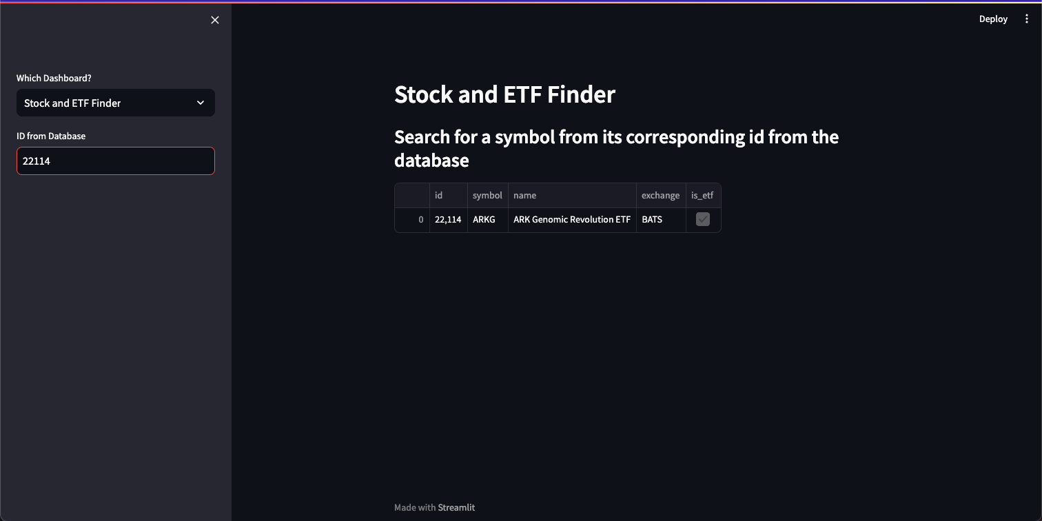
Stock Finder: Retrieves stock data based on the ID provided.
ETF List and Stock List: Fetches data directly from the respective database tables.
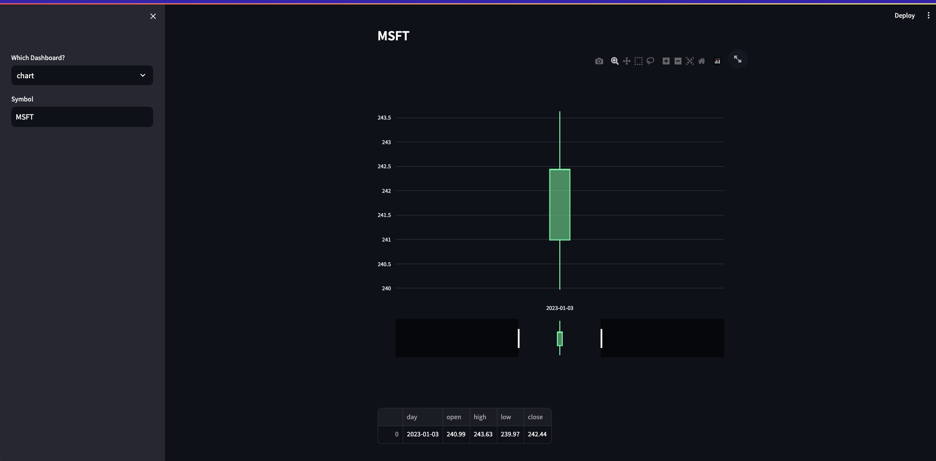
Chart: Generates a candlestick chart using Plotly based on the selected stock symbol.
Pattern: Performs different pattern-based analyses like hourly, daily, and 20 minute bars, moving averages, engulfing patterns, and three-bar patterns. It executes SQL queries to identify patterns and, if found, displays related images.

Data Retrieval and Visualization

The code utilizes SQL queries through pd.read_sql to retrieve data from the database based on user inputs. For instance, it fetches stock data for the chart and specific patterns based on symbol, time intervals, or pattern types. The queries are the same for each pattern as explained above.

if option == 'Stock Finder':
    st.subheader('Search for a stock symbol from its corresponding id from the database')
    id = st.sidebar.text_input("ID from Database", value='22114', max_chars=None, key=None, type='default')
    data = pd.read_sql(f"""select * from stock where id = {id} ;""", 
                            connection, params=(id.upper(),))
    st.write(data) 

if option == 'Etf List':
    data = pd.read_sql("select * from etf_holding;", connection)
    st.write(data)

if option == 'chart':
    symbol = st.sidebar.text_input("Symbol", value='MSFT', max_chars=None, key=None, type='default')

    data = pd.read_sql("""
        select date(day) as day, open, high, low, close
        from daily_bars
        where stock_id = (select id from stock where UPPER(symbol) = %s) 
        order by day asc""", connection, params=(symbol.upper(),))

    st.subheader(symbol.upper())

    fig = go.Figure(data=[go.Candlestick(x=data['day'],
                    open=data['open'],
                    high=data['high'],
                    low=data['low'],
                    close=data['close'],
                    name=symbol)])

    fig.update_xaxes(type='category')
    fig.update_layout(height=700)

    st.plotly_chart(fig, use_container_width=True)

    st.write(data)

if option == 'Stock List':
    data = pd.read_sql("select * from stock_price", connection)
    st.write(data)

if option == 'pattern':
    pattern = st.sidebar.selectbox(
        "Which Pattern?",
        ("1 Hour Price Bars","20 Minute Price Bars","Daily Moving Average","engulfing", "threebar")
    )

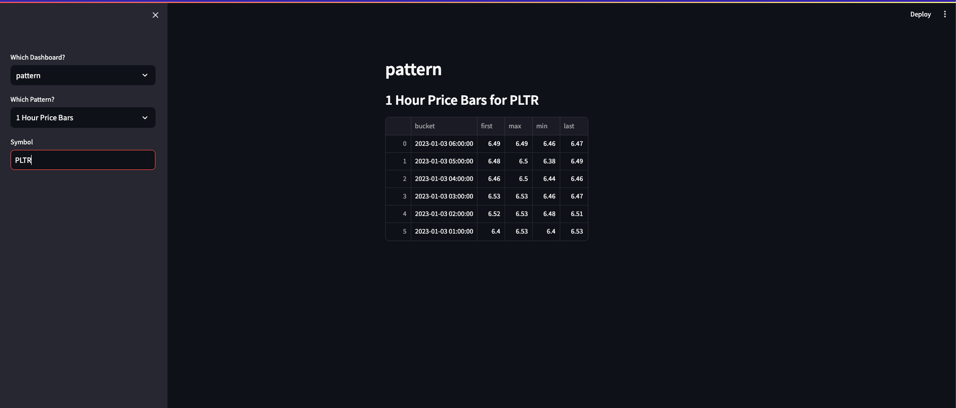
    if pattern == "1 Hour Price Bars":
        symbol = st.sidebar.text_input("Symbol", value='MSFT', max_chars=None, key=None, type='default')
        st.subheader(f'1 Hour Price Bars for {symbol}')
        data = pd.read_sql("""select time_bucket(INTERVAL '1 hour', dt) AS bucket, first(open, 
                                dt), max(high), min(low), last(close, dt) 
                                from stock_price 
                                where stock_id = (select id from stock where UPPER(symbol) = %s) 
                                group by bucket order by bucket desc;""", connection, params=(symbol.upper(),))
        st.write(data)

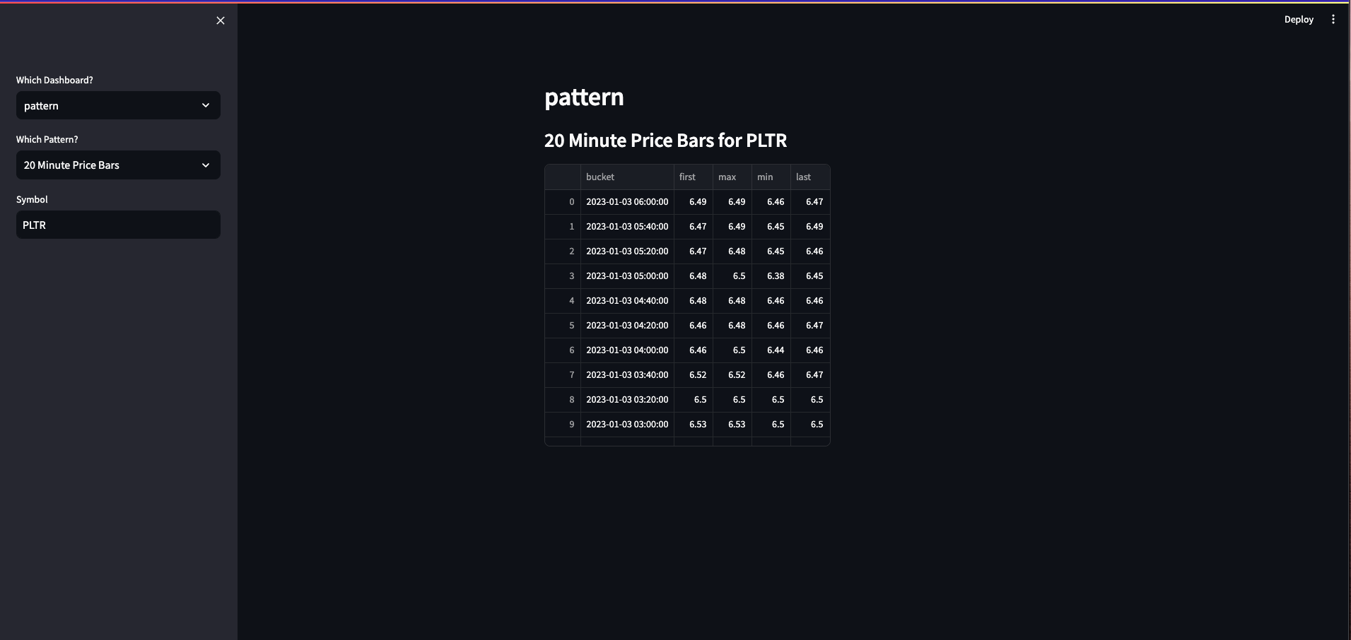
    if pattern == "20 Minute Price Bars":
        symbol = st.sidebar.text_input("Symbol", value='MSFT', max_chars=None, key=None, type='default')
        st.subheader(f'20 Minute Price Bars for {symbol}')
        data = pd.read_sql("""select time_bucket(INTERVAL '20 minute', dt) AS bucket, first(open, 
                                dt), max(high), min(low), last(close, dt) 
                                from stock_price 
                                where stock_id = (select id from stock where UPPER(symbol) = %s) 
                                group by bucket order by bucket desc;""", connection, params=(symbol.upper(),))
        st.write(data)

    if pattern == "Daily Moving Average":
        symbol = st.sidebar.text_input("Symbol", value='MSFT', max_chars=None, key=None, type='default')
        st.subheader(f'Daily Moving Average for {symbol}')
        data = pd.read_sql("""SELECT avg(close) FROM ( SELECT * FROM daily_bars where stock_id = (select id from stock where UPPER(symbol) = %s) 
                                    ORDER BY day DESC LIMIT 20 ) a;""", connection, params=(symbol.upper(),))
        st.write(data)

    if pattern == 'engulfing':
        cursor.execute("""
            SELECT * 
            FROM ( 
                SELECT day, open, close, stock_id, symbol, 
                LAG(close, 1) OVER ( PARTITION BY stock_id ORDER BY day ) previous_close, 
                LAG(open, 1) OVER ( PARTITION BY stock_id ORDER BY day ) previous_open 
                FROM daily_bars
                JOIN stock ON stock.id = daily_bars.stock_id
            ) a 
            WHERE previous_close < previous_open AND close > previous_open AND open < previous_close
            AND day = '2021-02-18'
        """)

    if pattern == 'threebar':
        cursor.execute("""
            SELECT * 
            FROM ( 
                SELECT day, close, volume, stock_id, symbol, 
                LAG(close, 1) OVER ( PARTITION BY stock_id ORDER BY day ) previous_close, 
                LAG(volume, 1) OVER ( PARTITION BY stock_id ORDER BY day ) previous_volume, 
                LAG(close, 2) OVER ( PARTITION BY stock_id ORDER BY day ) previous_previous_close, 
                LAG(volume, 2) OVER ( PARTITION BY stock_id ORDER BY day ) previous_previous_volume, 
                LAG(close, 3) OVER ( PARTITION BY stock_id ORDER BY day ) previous_previous_previous_close, 
                LAG(volume, 3) OVER ( PARTITION BY stock_id ORDER BY day ) previous_previous_previous_volume 
            FROM daily_bars 
            JOIN stock ON stock.id = daily_bars.stock_id) a 
            WHERE close > previous_previous_previous_close 
                AND previous_close < previous_previous_close 
                AND previous_close < previous_previous_previous_close 
                AND volume > previous_volume 
                AND previous_volume < previous_previous_volume 
                AND previous_previous_volume < previous_previous_previous_volume 
                AND day = '2021-02-19'
        """)

    try:
        rows = cursor.fetchall()

        for row in rows:
            st.image(f"https://finviz.com/chart.ashx?t={row['symbol']}")
    except psycopg2.ProgrammingError as e:
        st.subheader('')

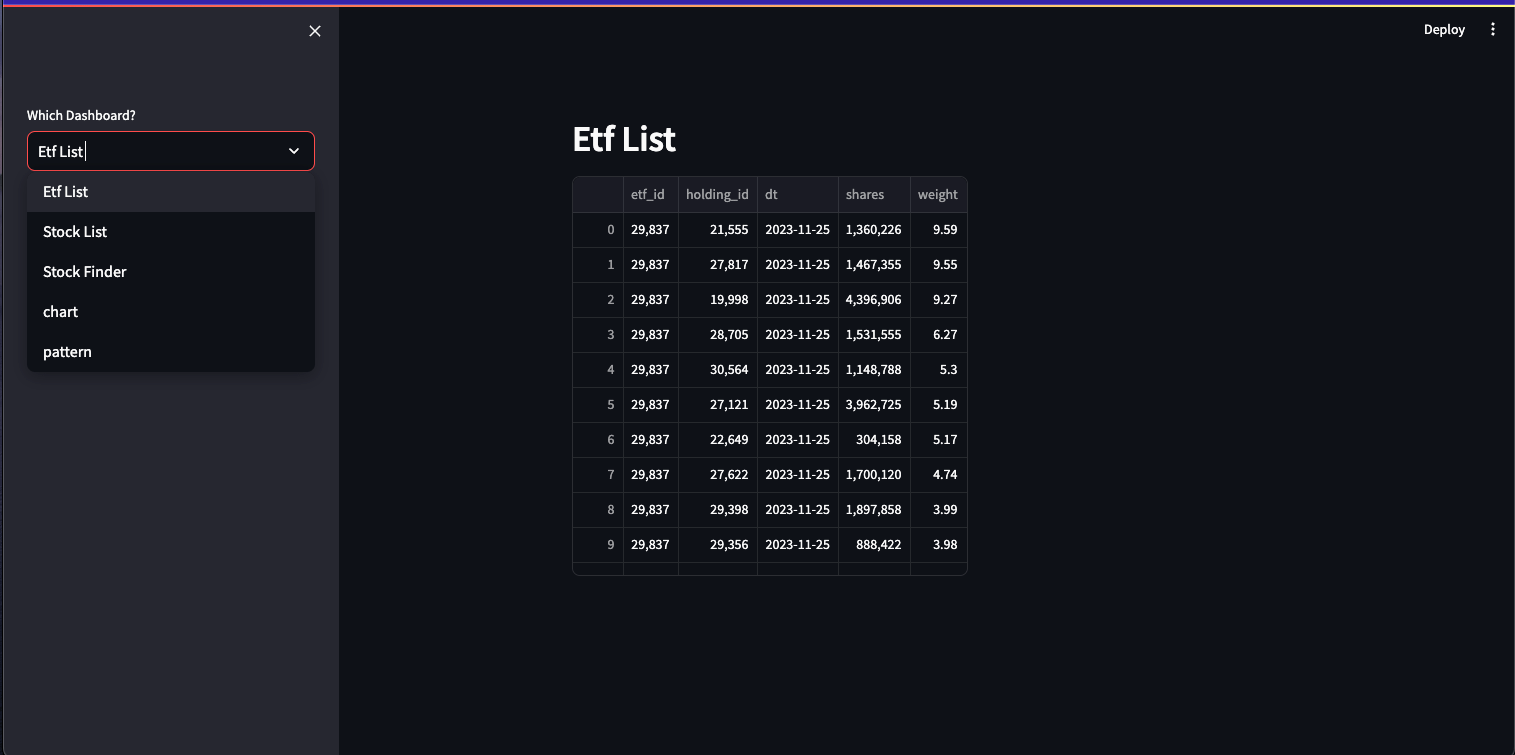
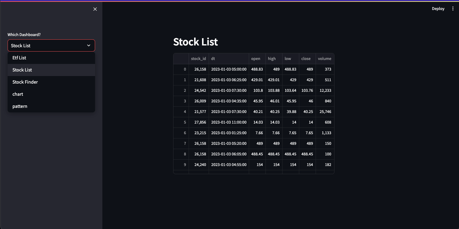
The following are screenshots of the dashboard. It allows users to select which dashboard and pattern from the dropdown menus on the left.

If applicable, it also allows you to search for a specific symbol stored in the database using the text input field.

Conclusion

I initially took on this project to explore an interesting trend I observed in some of my favourite ETFs, however after completing it I got to learn more about setting up and populating various types of databases, interfacing with and populating/updating said databases, and writing technical analysis queries.

I also got the chance to explore different technologies and methods such as Docker images, the pros and cons of dedicated time series databases compared to vanilla Postgres, and a more in-depth understanding of writing async coroutines and functions to build more efficient data loading implementations.

Gurik’s Substack

Ready for more?